Hash Tables

A hash table is an unordered collection of key-value pairs, where each key is unique. Also, they are the most commonly used data structure for implementing associative arrays¹ (maps, dictionaries).

“If I were stranded on a desert island and could only take one data structure with me, it would be the hash table.”

Peter Van Der Linden, from the book “Expert C Programming: Deep C Secrets”

They are so useful that, in most of the programming languages, there is a built-in hash table implementation of the standard library. It has different names in different programming languages. In some languages, it is called a dictionary, in some others it is called map or hash.

Language	Name of Hash Table
Java	HashMap, ConcurrentHashMap, HashTable
Python	dict
C++	std::unordered_map
C#	Dictionary, Hashtable
Ruby	Hash

Hash Table offers a combination of efficient O(1) complexity for average and amortized case² and O(N) complexity for worst case for insert, lookup and delete operations. Neither arrays or linked lists can achieve this. Each position of the hash table, often called a slot, can hold an item and is named by an integer value starting at 0.

Hash Function

The mapping between an item and the slot where that item belongs in the hash table is called the hash function. The hash function will take any item in the collection and return an integer in the range of slot names, between 0 and length-1.

When you are writing a hash function your main goal is that all the hashes would be distributed uniformly. To ensure this uniform distribution, our first strategy will be remainder method, which simply takes an item and divides it by the table size, returning the remainder as its hash value.

Assume that we have a hash table with the size 13, and the set of integer items 99, 17, 54, 26, 75, 31, and 50.

If we apply remainder method to 99, with the formula: hash = item % len(hash_table), the remainder will be 8. If we apply the same formula to all items;

Item	Hash Value
99	8
17	4
54	2
26	0
75	10
31	5
50	11

Visualization of the table would be;

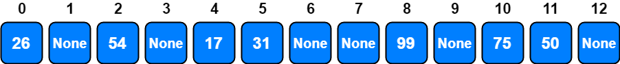
Load Factor represents the load on our hash table. It is a good way to understand how much full our hash table is. If there are n entries, than load_factor = n / sizeoftable. In our case, it is 7 / 13.

As you can see, all items are uniformly distributed. But using remainder method does not guarantee avoiding potential collisions. For example, if there was an item, 69 in the list, the remainder is 4 and this means that there would be a collision between item 17 and item 69.

Choosing a Good Hash Function

Given a collection of items, a hash function that successfully maps each item into a unique slot is referred to as a perfect hash function. In reality, constructing a perfect hash is only possible when we are sure that the items and the collection will never change. Otherwise, given an arbitrary collection of items, there is no systematic way to construct a perfect hash function. Luckily, we do not need the hash function to be perfect to still gain performance efficiency.

One way to always have a perfect hash function is to increase the size of the hash table so that each possible value in the item range can be accommodated. This guarantees that each item will have a unique slot. Although this is practical for small numbers of items, it is not feasible when the number of possible items is large. For example, if the items were nine-digit Social Security numbers, this method would require almost one billion slots. If we only want to store data for a class of 25 students, we will be wasting an enormous amount of memory.

Another technique to create hash functions is mid-square method. We first square the item, and then extract some portion of the resulting digits. If the result has fewer than 2n digits, leading zeroes are added to compensate; the middle n digits of the result would be the next number in the sequence, and returned as the result.

For example, if the item were 99, we would first compute 99² = 9801. By extracting the middle two digits, 80, and performing the remainder step, we get 2 = (80 % 13).

Item	Remainder	Mid-square
99	8	2
17	4	2
54	2	0
26	0	2
75	10	10
31	5	5
50	11	11
69	4	11

As you can see, collisions are hard to avoid so, we need to find a way to resolve possible collisions.

Collision Resolution

When two items hash to the same slot, we must have a systematic method for placing the second item in the hash table. This process is called collision resolution.³

Open Addressing

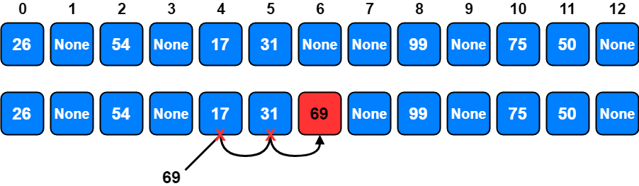
One method for resolving collisions looks into the hash table and tries to find another open slot to hold the item that caused the collision. A simple way to do this is to start at the original hash value position and then move in a sequential manner through the slots until we encounter the first slot that is empty.

Note that we may need to go back to the first slot (circularly) to cover the entire hash table. This collision resolution process is referred to as open addressing in that it tries to find the next open slot or address in the hash table. By systematically visiting each slot one at a time, we are performing an open addressing technique called linear probing.

For example with the remainder method we said that, if there was an item, 69 in the list, the remainder is 4 and this means that there would be a collision between item 17 and item 69 at position 4. To solve this collision with linear probing method, we are going to try the next slot, 5 which is also occupied. So, we are going to try one more, and will find an empty slot at position 6.

The general name for this process of looking for another slot after a collision is rehashing.

The plus 3 rehash method can be defined as rehash(pos) = (pos + skip) % sizeoftable where skip = 3. It is important to note that the size of the skip must be such that all the slots in the table will eventually be visited. Otherwise, part of the table will be unused. To ensure this, it is often suggested that the table size be a prime number. This is the reason we have been using 13 in our examples.

A variation of the linear probing idea is called quadratic probing. Instead of using a constant skip value, we use a rehash function that increments the hash value by 1, 3, 5, 7, 9, and so on. This means that if the first hash value is h, the successive values are h + 1, (h + 1) + 3 = h + 4, (h + 4) + 5 = h + 9, (h + 9) + 7 = h + 16 and so on. In other words, quadratic probing uses a skip consisting of successive perfect squares.

Double hashing⁴ is similar to linear probing and the only difference is the interval between successive probes. Here, the interval between probes is computed by using two hash functions.

(hash1(key) + (pos * hash2(key))) % sizeoftable formula can be used for double hashing.

First hash function is typically; hash1(key) = key % sizeoftable

And a popular second hash function is; hash2(key) = prime - (key % prime) where prime is a prime number smaller than the sizeoftable.

There are also other Open Adressing hashing methods like Cuckoo hashing, Coalesced hashing, Hopscotch hashing, Robin Hood hashing, 2-choice hashing etc. but it would be too much to explain all of them in this article.

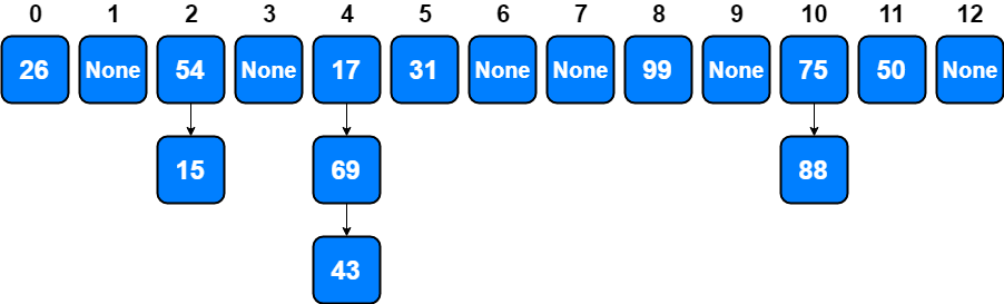
Chaining

An alternative method for handling the collision problem is to allow each slot to hold a reference to a collection (or chain) of items. Chaining allows many items to exist at the same location in the hash table. When collisions happen, the item is still placed in the proper slot of the hash table. As more and more items hash to the same location, the difficulty of searching for the item in the collection increases.

Lets go back to remainder example where adding 69 was creating a collision between 17 and 69 at slot 4. Adding 43 is another collision at slot 4. Also, 15 and 88 create collisions at slots 2 and 10 respectively.

We can represent this situation with chaining as below.

When we want to search for an item, we use the hash function to generate the slot where it should reside. Since each slot holds a collection, we use a searching technique to decide whether the item is present. The advantage is that on the average there are likely to be many fewer items in each slot, so the search is perhaps more efficient.

Implementation

Lets summarize all of them with a complete Python Hash Table implementation.

class HashTable:
    def __init__(self):
        self.size = 13
        self.slots = [None] * self.size
        self.data = [None] * self.size

    def put(self, key, data):
        hash_value = self.hashfunction(key, len(self.slots))

        if self.slots[hash_value] is None:
            self.slots[hash_value] = key
            self.data[hash_value] = data
        else:
            if self.slots[hash_value] == key:
                self.data[hash_value] = data
            else:
                next_slot = self.rehash(hash_value, len(self.slots))
                while self.slots[next_slot] is not None and self.slots[next_slot] != key:
                    next_slot = self.rehash(next_slot, len(self.slots))

                if self.slots[next_slot] is None:
                    self.slots[next_slot] = key
                    self.data[next_slot] = data
                else:
                    self.data[next_slot] = data

    def hashfunction(self, key, size):
        return key % size  # remainder method

    def rehash(self, old_hash, size):
        return (old_hash + 1) % size  # linear probing

    def get(self, key):
        start_slot = self.hashfunction(key, len(self.slots))

        data = None
        stop = False
        found = False
        position = start_slot
        while self.slots[position] is not None and not found and not stop:
            if self.slots[position] == key:
                found = True
                data = self.data[position]
            else:
                position = self.rehash(position, len(self.slots))
                if position == start_slot:
                    stop = True
        return data

    def __getitem__(self, key):
        return self.get(key)

    def __setitem__(self, key, data):
        self.put(key, data)

Now we can try our HashTable() implementation together.

hash_table = HashTable()
hash_table[99] = "cat"
hash_table[17] = "dog"
hash_table[54] = "lion"
hash_table[26] = "tiger"
hash_table[75] = "bird"
hash_table[31] = "cow"
hash_table[50] = "goat"
hash_table[69] = "pig"

print(hash_table.slots)
# Output: [26, None, 54, None, 17, 31, 69, None, 99, None, 75, 50, None]

print(hash_table.data)
# Output: ['tiger', None, 'lion', None, 'dog', 'cow', 'pig', None, 'cat', None, 'bird', 'goat', None]

References

1. Wikipedia, Associative Array
2. Wikipedia, Amortized analysis
3. Problem Solving with Algorithms and Data Structures using Python, Collision Resolution
4. Wikipedia, Double Hashing