Dynamic Programming

Dynamic programming is all about breaking down an optimization problem into simpler sub-problems, and storing the solution to each sub-problem so that each sub-problem is solved only once.

This method was developed by Richard Bellman in the 1950s. He explained the reasoning behind the name “Dynamic Programming” in his autobiography¹ and the main reason was: “to pick a term that didn’t sound like mathematical research”.

He wrote that the Secretary of Defense at the time was biased against research. So he picked “programming”, which sounded less like research. He also wanted to get across the idea that it was multistage, so he picked “dynamic”. The final name was also hard to use in a negative way, even for a Congressman!

Sub-problems

We said that, it is all about breaking down the original problem into simpler sub-problems. But what is a sub-problem?

For example lets think about a simple mathematical calculation:

3 + 7 + 8 + 1 + 5 + 2 + 3 + 7 + 8 + 8 + 8 + 1 = 61

We can divide it into sub-problems;

3 + 7 = 10
8 + 1 = 9
5 + 2 = 7
3 + 7 ---> We already calcualted it! It's 10.
8 + 8 = 16
8 + 1 ---> We already calcualted it! It's 9.

In Dynamic Programming (DP), we are storing the solutions of sub-problems so that we do not need to recalculate it later. This is called Memoization.

By finding the solutions for every single sub-problem, we can solve the original problem itself.

Memoization

Memoization refers to the technique of caching and reusing previously computed results. It is a top-down approach where we just start by solving the problem in a natural manner and storing the solutions of the sub-problems along the way.

Suppose that we want to find the Fibonacci number at a particular index of the sequence. So fibonacci(n) = n^th element in the Fibonacci sequence.

This problem is normally solved with Divide and Conquer algorithm. There are 3 main parts in this technique:

1. Divide - divide the problem into smaller sub-problems of the same type
2. Conquer - solve the sub-problems recursively
3. Combine - combine all the sub-problems to create a solution to the original problem

Lets define a function which will be responsible for calculating each of the Fibonacci numbers up to some defined limit n.

def fibonacci(n):
    if n == 0 or n == 1:
        return n
    else:
        return fibonacci(n - 1) + fibonacci(n - 2)

This first naive solution recursively calculates each number in the sequence from scratch. This method has O(2ⁿ) time complexity, which is really bad runetime. For example, calculating fibonacci(40) will take more than a minute!

This also happens to be a good example of the danger of naive recursive functions.

The main idea behind Memoization was to re-use already calculated sub-problem results in order to solve the original problem.

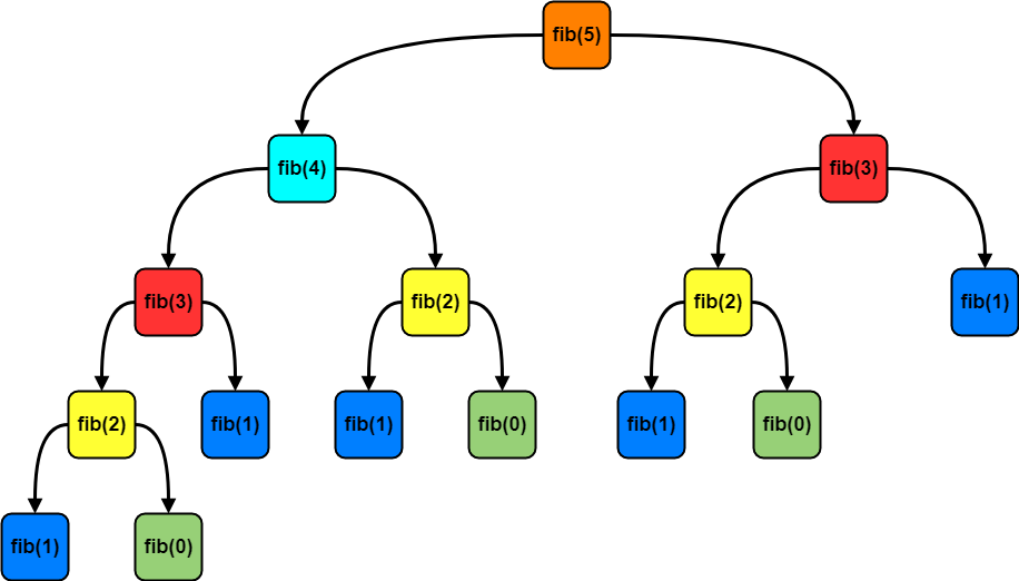
As you can see in the recursion tree, the same sub-problems occured more than once. For example fib(3) is occuring twice, fib(2) is occuring 3 times etc.

So, despite calculating the result of the same problem, again and again, we can store the results once and use them again whenever needed.

Let’s write the same code but this time by storing the terms we have already calculated.

memo = {0: 0, 1: 1}

def fibonacci_memoization(n):
    if n in memo.keys():
        return memo[n]
    else:
        memo[n] = fibonacci_memoization(n - 1) + fibonacci_memoization(n - 2)
        return memo[n]

By not computing the full recusrive tree on each iteration, we’ve essentially reduced the running time for fibonacci(40) from more than a minute to almost instant. But we are sacrificing memory for the speed. Dynamic programming basically trades time with memory.

Tabulation

The other way we could have solved the Fibonacci problem was by starting from the bottom i.e., start by calculating the 2^nd term and then 3^rd and so on and finally calculating the higher terms on the top of these, by using these values. This bottom-up approach is called Tabulation.

def fibonacci_tabulation(n):
    if n == 0:
        return n

	# pre-initialize array
    f = [0] * (n + 1)
    f[1] = 1

    for i in range(2, n + 1):
        f[i] = f[i - 1] + f[i - 2]
    return f[n]

Memoization vs Tabulation

Generally speaking, memoization is easier to code than tabulation. We can write a memoriser wrapper function that automatically does it for us. With tabulation, we have to come up with an ordering.

Also, memoization is indeed the natural way of solving a problem, so coding is easier in memoization when we deal with a complex problem. Coming up with a specific order while dealing with lot of conditions might be difficult in the tabulation.

What is more, think about a case when we don’t need to find the solutions of all the subproblems. In that case, we would prefer to use the memoization instead.

Tabulation is faster, as you already know the order and dimensions of the table. Memoization is slower, because you are creating the table on the fly. Generally, memoization is also slower than tabulation because of the large recursive calls.

In memoization, table does not have to be fully computed, it is just a cache while in tabulation, table is fully computed.

If all sub-problems must be solved at least once, a bottom-up tabulated dynamic programming algorithm usually outperforms a top-down memoized algorithm by a constant factor.

References

1. Wikipedia, Eye of the Hurricane: An Autobiography, (1984, page 159)
2. Wikipedia, Dynamic Programming
3. Wikipedia, Memoization