Sorting Algorithms with Animations

Sorting refers to arranging the given data in a particular format and it is one of the most common operations in Computer Science.

The different sorting algorithms are a perfect showcase of how algorithm design can have such a strong effect on program complexity, speed, and efficiency. So, I will attempt to describe some of the most popular sorting methods and highlight their benefits and shortcomings with using animations and Python code implementations of them.

All animations in this post is generated with Timo Bingmann’s awesome tiny program called Sound of Sorting¹. Generated animations turned into gif images by myself.

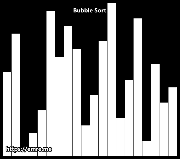
Bubble Sort

Bubble sort is the one usually taught in introductory Computer Science classes since it clearly demonstrates how sort works while being simple and easy to understand.

We begin by comparing the first two elements of the list. If the first element is larger than the second element, we swap them. If they are already in order we leave them as is. We then move to the next pair of elements, compare their values and swap as necessary. This process continues to the last pair of items in the list.

Implementation

def bubble_sort(array):
    # We set swapped to True so the loop runs at least once
    swapped = True

    while swapped:
        swapped = False
        for i in range(len(array) - 1):
            if array[i] > array[i + 1]:
                # Swap the elements
                array[i], array[i + 1] = array[i + 1], array[i]
                # Set the flag to True so we'll loop again
                swapped = True

    return array

Selection Sort

Selection sort is also quite simple but frequently outperforms Bubble sort. This algorithm segments the list into two parts: sorted and unsorted.

We first find the smallest element in the unsorted sublist and place it at the end of the sorted sublist. Thus, we continuously remove the smallest element of the unsorted sublist and append it to the sorted sublist. This process continues iteratively until the list is fully sorted.

Implementation

def selection_sort(array):
    for i in range(len(array)):
        # We assume that the first item of the unsorted segment is the smallest
        min_value = i

        for j in range(i + 1, len(array)):
            if array[j] < array[min_value]:
                min_value = j

        # Swap values of the lowest unsorted element with the first unsorted element
        array[i], array[min_value] = array[min_value], array[i]

    return array

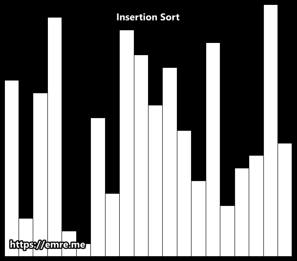
Insertion Sort

Insertion sort is a simple sorting algorithm that works the way we sort playing cards in our hands. It is both faster and simpler than both Bubble sort and Selection sort.

Like Selection sort, this algorithm segments the list into sorted and unsorted parts. It iterates over the unsorted sublist, and inserts the element being viewed into the correct position of the sorted sublist. It repeats this process until no input elements remain.

Implementation

def insertion_sort(array):
    # We assume that the first item is sorted
    for i in range(1, len(array)):
        picked_item = array[i]

        # Reference of the index of the previous element
        j = i - 1

        # Move all items to the right until finding the correct position
        while j >= 0 and array[j] > picked_item:
            array[j + 1] = array[j]
            j -= 1

        # Insert the item
        array[j + 1] = picked_item

    return array

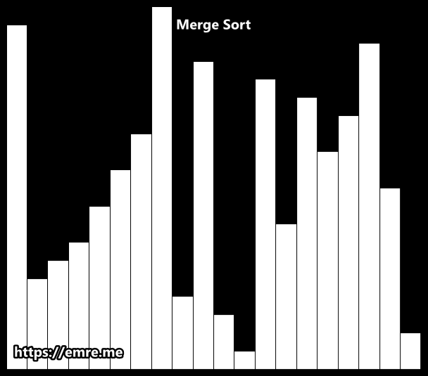
Merge Sort

Merge sort is a very good example of Divide and Conquer² algorithms. We recursively split the list in half until we have lists with size one. We then merge each half that was split, sorting them in the process.

Sorting is done by comparing the smallest elements of each half. The first element of each list are the first to be compared. If the first half begins with a smaller value, then we add that to the sorted list.

Implementation

def merge_sort(array):
    # If the list is a single element, return it
    if len(array) <= 1:
        return array

    mid = len(array) // 2

    # Recursively sort and merge each half
    l_list = merge_sort(array[:mid])
    r_list = merge_sort(array[mid:])

    # Merge the sorted lists into a new one
    return _merge(l_list, r_list)


def _merge(l_list, r_list):
    result = []
    l_index, r_index = 0, 0

    for i in range(len(l_list) + len(r_list)):
        if l_index < len(l_list) and r_index < len(r_list):

            # If the item at the beginning of the left list is smaller, add it to the sorted list
            if l_list[l_index] <= r_list[r_index]:
                result.append(l_list[l_index])
                l_index += 1

            # If the item at the beginning of the right list is smaller, add it to the sorted list
            else:
                result.append(r_list[r_index])
                r_index += 1

        # If we have reached the end of the of the left list, add the elements from the right list
        elif l_index == len(l_list):
            result.append(r_list[r_index])
            r_index += 1

        # If we have reached the end of the of the right list, add the elements from the left list
        elif r_index == len(r_list):
            result.append(l_list[l_index])
            l_index += 1

    return result

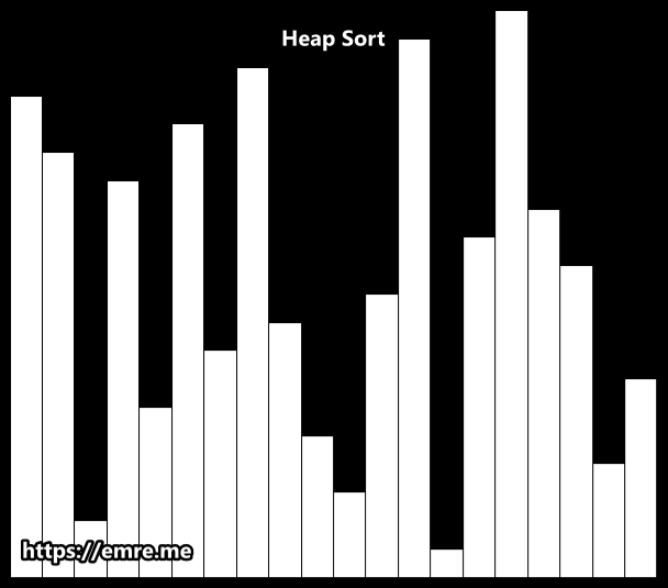
Heap Sort

Heap sort is the improved version of the Selection sort, which takes advantage of a heap data structure rather than a linear-time search to find the max value item.

Using the heap, finding the next largest element takes O(log(n)) time, instead of O(n) for a linear scan as in simple selection sort. This allows heap sort to run in O(n log(n)) time, and this is also the worst case complexity.

Implementation

We already know how to create a max heap. If you can’t remember, you can read about it in Heaps data structure article. First part of the code where we are defining max_heapify() will be a copy/paste from this article.

def get_left_child(i):
    return 2 * i + 1


def get_right_child(i):
    return 2 * i + 2


def max_heapify(arr, n, i):
    left = get_left_child(i)
    right = get_right_child(i)
    largest = i

    if left < n and arr[left] > arr[largest]:
        largest = left
    if right < n and arr[right] > arr[largest]:
        largest = right
    if largest != i:
        arr[i], arr[largest] = arr[largest], arr[i]
        max_heapify(arr, n, largest)


def heap_sort(arr):
    n = len(arr)

    # build the max heap
    for i in range(n, -1, -1):
        max_heapify(arr, n, i)

    # extract elements one by one
    for i in range(n - 1, 0, -1):
        arr[i], arr[0] = arr[0], arr[i]
        max_heapify(arr, i, 0)

    return arr

Luckly, there is also a built-in Python library called heapq and we can implement Heap Sort very simply with using this library too.

import heapq

def heap_sort(array):
    h = []
    for value in array:
        heapq.heappush(h, value)
    return [heapq.heappop(h) for i in range(len(h))]

Quick Sort

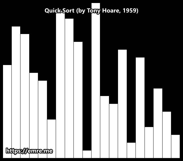
Quick sort is developed by British computer scientist Tony Hoare in 1959. It is still a commonly used algorithm for sorting. When implemented well, it can be about two or three times faster than its main competitors, merge sort and heap sort.

The quick sort uses divide and conquer to gain the same advantages as the merge sort, while not using additional storage. As a trade-off, however, it is possible that the list may not be divided in half. When this happens, we will see that performance is diminished.

It has 3 steps:

1. We first select an element which we will call the pivot from the array.
2. Move all elements that are smaller than the pivot to the left of the pivot; move all elements that are larger than the pivot to the right of the pivot. This is called the partition operation.
3. Recursively apply the above 2 steps separately to each of the sub-arrays of elements with smaller and bigger values than the last pivot.

Choice of Pivot

Selecting a good pivot value is key to efficiency. There are different strategies to select the pivot, which are;

1. Picking the first element as pivot
2. Picking the last element as pivot
3. Picking a random element as pivot
4. Picking the median as pivot
5. Applying “median-of-three” rule (recommended by Sedgewick) which you look at the first, middle and last elements of the array, and choose the median of those three elements as the pivot.

Hoare partition scheme

Hoare partition scheme uses two indices that start at the ends of the array being partitioned, then move toward each other, until they detect an inversion: a pair of elements, one greater than or equal to the pivot, one lesser or equal, that are in the wrong order relative to each other. The inverted elements are then swapped. When the indices meet, the algorithm stops and returns the final index.

Hoare’s scheme is more efficient than Lomuto’s partition scheme because it does three times fewer swaps on average.

Implementation (Hoare)

def partition(array, low, high):
    # We select the middle element to be the pivot
    pivot = array[(low + high) // 2]
    i = low - 1
    j = high + 1
    while True:
        i += 1
        while array[i] < pivot:
            i += 1

        j -= 1
        while array[j] > pivot:
            j -= 1

        if i >= j:
            return j

        # Swap
        array[i], array[j] = array[j], array[i]


def quick_sort(array):
    quick_sort_helper(array, 0, len(array) - 1)


def quick_sort_helper(items, low, high):
    if low < high:
        split_point = partition(items, low, high)
        quick_sort_helper(items, low, split_point)
        quick_sort_helper(items, split_point + 1, high)

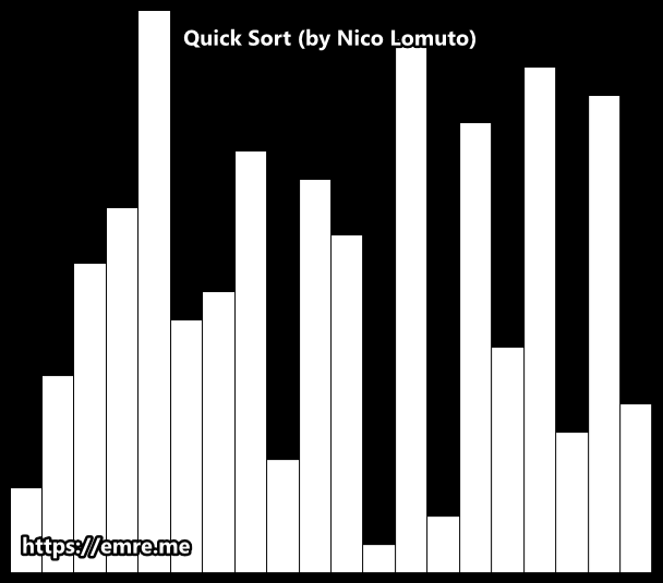
Lomuto partition scheme

This scheme is attributed to Nico Lomuto and popularized by Jon Bentley in his book Programming Pearls and Thomas H. Cormen in their book Introduction to Algorithms.

This scheme chooses a pivot that is typically the last element in the array. The algorithm maintains index i as it scans the array using another index j such that the elements low through i-1 (inclusive) are less than the pivot, and the elements i through j (inclusive) are equal to or greater than the pivot.

As this scheme is more compact and easy to understand, it is frequently used in introductory material, although it is less efficient than Hoare’s original scheme. This scheme degrades to O(n²) when the array is already in order.

Implementation (Lomuto)

def partition(array, low, high):
    pivot = array[high]

    i = low
    j = low
    while j < high:
        if array[j] <= pivot:
            array[i], array[j] = array[j], array[i]
            i += 1

        j += 1

    # swap
    array[i], array[high] = array[high], array[i]

    return i


def quick_sort(array):
    quick_sort_helper(array, 0, len(array) - 1)


def quick_sort_helper(items, low, high):
    if low < high:
        split_point = partition(items, low, high)
        quick_sort_helper(items, low, split_point - 1)
        quick_sort_helper(items, split_point + 1, high)

Python’s Built-in Sort Functions

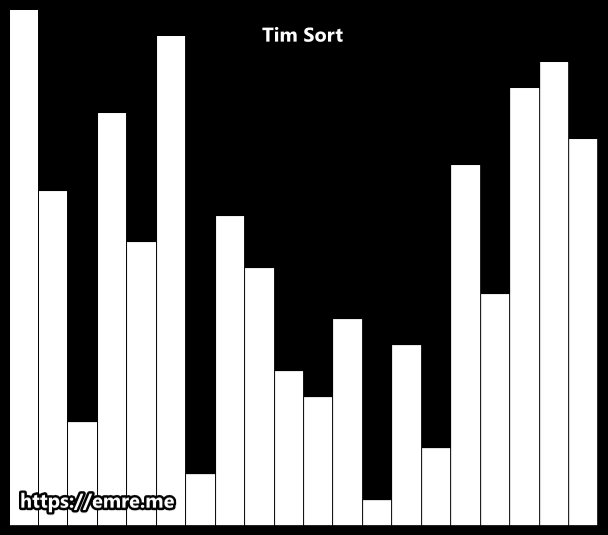
While it’s beneficial to understand these sorting algorithms, in most Python projects you would probably use the sort functions already provided in the language.

These sort functions implement the Tim Sort algorithm, which is based on Merge Sort and Insertion Sort.

sort()

We can change our list to have it’s contents sorted with the sort() method:

arr = [4, 7, 224, 19, 1, 5, 3, 10, 187, 13, 2]
arr.sort()

print(arr)
# Output: [1, 2, 3, 4, 5, 7, 10, 13, 19, 187, 224]

arr.sort(reverse=True)

print(arr)
# Output: [224, 187, 19, 13, 10, 7, 5, 4, 3, 2, 1]

sorted()

The sorted() function can sort any iterable object, that includes - lists, strings, tuples, dictionaries, sets, and custom iterators you can create.

arr = [4, 7, 224, 19, 1, 5, 3, 10, 187, 13, 2]
sorted_arr = sorted(arr)

print(sorted_arr)
# Output: [1, 2, 3, 4, 5, 7, 10, 13, 19, 187, 224]
 
reverse_sorted_arr = sorted(arr, reverse=True)

print(reverse_sorted_arr)
# Output: [224, 187, 19, 13, 10, 7, 5, 4, 3, 2, 1]

Stable vs Unstable Algorithms

A sorting algorithm is said to be stable if two objects with equal keys appear in the same order in the sorted output as they appear in the unsorted input.

Whereas a sorting algorithm is said to be unstable if there are two or more objects with equal keys which don’t appear in same order before and after sorting.

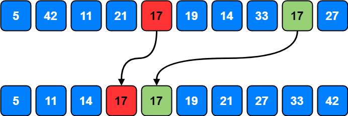
Bubble sort, Insertion sort, Merge sort etc. are stable by nature and other sorting algorithms like Quick sort, Heap sort are not stable by nature but can be made stable by taking the position of the elements into consideration.

Any sorting algorithm may be made stable, at a price: The price is O(n) extra space, and moderately increased running time (less than doubled, most likely). ^{3 4}

Time Complexities of Sorting Algorithms

If we are talking about algorithms, then the most important factor which affects our decision process is time and space complexity.

Algorithm	Time Complexity (Best)	Time Complexity (Average)	Time Complexity (Worst)	Space Complexity
Bubble Sort	O(n)	O(n2)	O(n2)	O(1)
Selection Sort	O(n2)	O(n2)	O(n2)	O(1)
Insertion Sort	O(n)	O(n2)	O(n2)	O(1)
Merge Sort	O(n log(n))	O(n log(n))	O(n log(n))	O(n)
Heap Sort	O(n log(n))	O(n log(n))	O(n log(n))	O(1)
Quick Sort	O(n log(n))	O(n log(n))	O(n2)	O(log(n))
Radix Sort	O (nk)	O(nk)	O(nk)	O(n+k)
Tim Sort	O(n)	O(n log(n))	O(n log(n))	O(n)

Which one should I choose?

It depends. Everything in Computer Science is a trade-off and sorting algorithms are no exception. Each algorithm comes with its own set of pros and cons.⁵

• Quick sort is a good default choice. It tends to be fast in practice, and with some small tweaks its dreaded O(n²) worst-case time complexity becomes very unlikely. A tried and true favorite.
• Heap sort is a good choice if you can’t tolerate a worst-case time complexity of O(n²) or need low space costs. The Linux kernel uses heap sort instead of quick sort for both of those reasons.
• Merge sort is a good choice if you want a stable sorting algorithm. Also, merge sort can easily be extended to handle data sets that can’t fit in RAM, where the bottleneck cost is reading and writing the input on disk, not comparing and swapping individual items.
• Radix sort looks fast, with its O(n) worst-case time complexity. But, if you’re using it to sort binary numbers, then there’s a hidden constant factor that’s usually 32 or 64 (depending on how many bits your numbers are). That’s often way bigger than O(log(n)), meaning radix sort tends to be slow in practice.

So you have to know what’s important in the problem you’re working on.

• How large is your input?
• How many distinct values are in your input?
• How much space overhead is acceptable?
• Can you afford O(n²) worst-case runtime?

Once you know what’s important, you can pick the sorting algorithm that does it best.

Other Sorting Algorithms

Sorting is a vast topic and it is not possible to cover every Sorting Algorithm in this single post. It is also very popular research topic in academia and people are coming up with new sorting algorithms every year.

There are also some funny ones coming from Reddit, like Stalin Sort⁶.

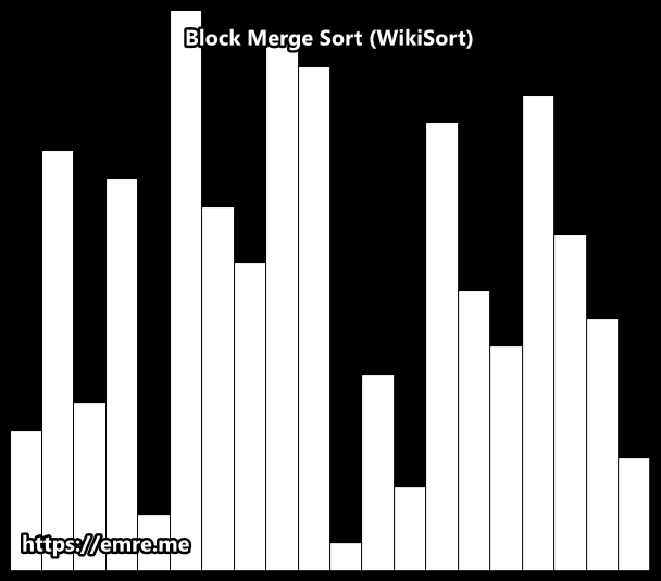
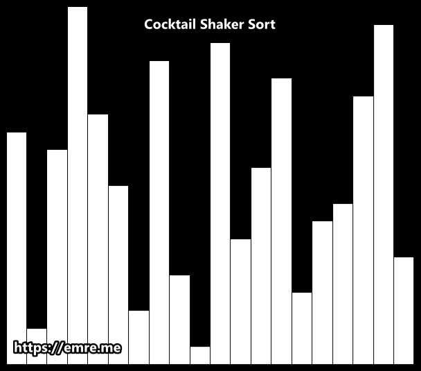
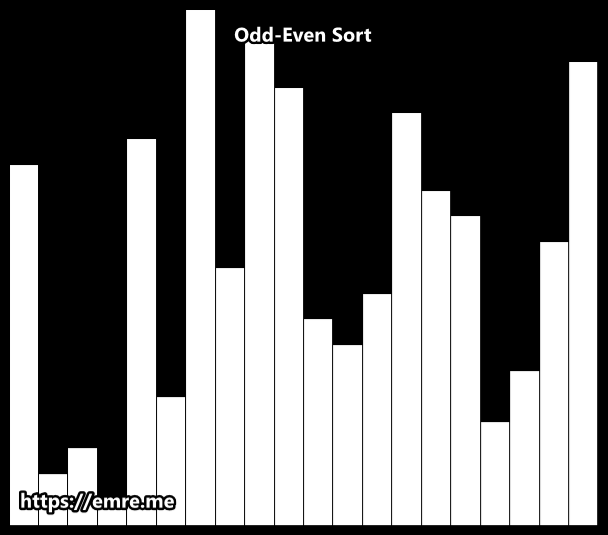
If you are curious, I created more animated gifs for;

• Bitonic Sort
• Block Merge Sort
• Cocktail Shaker Sort
• Comb Sort
• Cycle Sort
• Gnome Sort
• Odd-Even Sort
• Quick Sort - Bentley & Sedgewick
• Radix Sort - Least Significant Digit
• Radix Sort - Most Significant Digit
• Shell Sort
• Smooth Sort

For other algorithms which are not in the list, Wikipedia is your friend. Even the least known sorting algorithms have their dedicated wiki pages with some good explanation.

References

1. Timo Bingmann, Sound of Sorting
2. Wikipedia, Divide and Conquer algorithm
3. Wikipedia, Sorting Algorithm Stability
4. The University of Illinois at Chicago, CS MSc.401 - Stability
5. Interview Cake, Sorting Algorithm Cheat Sheet
6. Github/gustavo-depaula, Stalin Sort